Theory

T17

Search on the web about possible derivation of the Normal Distribution.

In statistics, a normal distribution or Gaussian distribution is a type of continuous probability distribution for a real-valued random variable. The general form of its probability density function is:

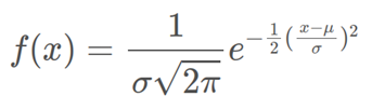
The parameter \mu is the mean of the distribution, while the parameter \sigma stands for its standard deviation. The variance of the distribution is \sigma ^{2}. A random variable with a Gaussian distribution is said to be normally distributed, and it is called a normal deviate.

Normal distributions are important in statistics and are often used in the natural and social sciences to represent real-valued random variables whose distributions are not known. Starting from the normal distribution we can study on different derivations of it:

Central limit theorem

Their importance is partly due to the central limit theorem. It states that, under some conditions, the average of many samples (observations) of a random variable with finite mean and variance is itself a random variable—whose distribution converges to a normal distribution as the number of samples increases. Therefore, physical quantities that are expected to be the sum of many independent processes, such as measurement errors, often have distributions that are nearly normal.

De Moivre

The origin of normal distribution can be traced to a French mathematician Abraham de Moivre. He had scientific interest in gambling and often acted as a consultant to gamblers to determine probabilities. De Moivre allegedly was studying the probability distribution of coin flips. He was trying to come up with a mathematical expression such as finding a probability of 60 or more tails out of one hundred coin flips. As an answer to this question he derived a bell shaped distribution which is commonly referred as the normal curve.

The theorem shows that the probability mass function of the random number of “successes” observed in a series of n independent Bernoulli trials, each having probability p of success (a binomial distribution with n trials), converges to the probability density function of the normal distribution with mean np and standard deviation sqrt{np*(1-p)}, as n grows large, assuming p is not 0 or 1.

THEOREM:

As n grows large, for k in the neighborhood of np we can approximate:

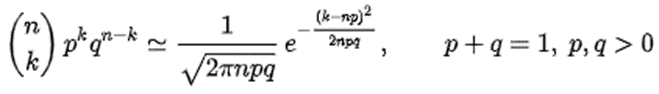
in the sense that the ratio of the left-hand side to the right-hand side converges to 1 as n → ∞.

T18

Search on the web about method to generate normal variate (eg Marsaglia method, etc.)

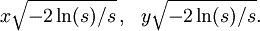
Marsaglia Polar Method

It is a method for generating a pair of independent standard normal random variables by choosing random points (x, y) in the square −1 < x < 1, −1 < y < 1 until we obtain: 0 < s = x^2 + y^2 < 1, And the pair of random variables:

Box-Muller Method

Another method that is also very easy to implement was introduced by Box-Muller (1958). This algorithm can be used for generating a pair of independent random variables from the standard normal distribution.

1. Generate two random numbers U1 and U2 from U(0,1).
2. Set V1 = U1 – 1, V2 = U1 – 1 and S = V21 – V22 (note that V1 and V2 are U(-1, 1).
3. If S > 1 go to step 1, otherwise go to step 4.
4. Return the independent standard normal variables:

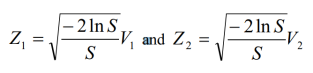
This algorithm also requires two uniform variables to generate a single standard normal variable.

Applications

A12

Consider R (radius), A(angle) uniform rv’s and use them as random polar coordinates on a plane. Determine the empirical distribution of the corresponding Cartesian coordinates (X,Y).

The proposed solution can be found at this GitHub link.

A13

Search for the methods to generate Normal rv’s X from uniform rv’s, and simulate the following distribution: X, X², X/Y², X²/Y², X/Y .

The proposed solution can be found at this GitHub link.

Research

TA7

Find in the web what are the distributions that you just simulated.

Normal Distribution(X)

We plot the distribution of one of our normal random variables by representing all the samples taken in a histogram. In the histogram we can see how the it resembles the density function of the normal distribution.

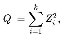
Chi-squared distribution

The chi-squared distribution is the distribution of a sum of the squares of k independent standard normal random variables. It’s used in the common chi-squared tests for goodness of fit of an observed distribution to a theoretical one, the independence of two criteria of classification of qualitative data, and in confidence interval estimation for a population standard deviation of a normal distribution from a sample standard deviation. Given Z1,…Zk independent, standard normal random variables is distributed according to the chi-squared distribution with k degrees of freedom, with the following formula:

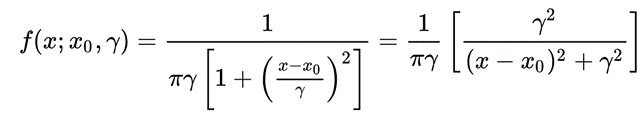
Cauchy Distribution

The Cauchy Distribution is is the distribution of the x-intercept of a ray issuing from (x0, gamma) with a uniformly distributed angle. It is also the distribution of the ratio of two independent normally distributed random variables with mean zero. Defined as:

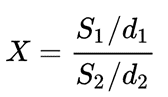
The Fisher Distribution

It is a continuous probability distribution that arises frequently as the null distribution of a test statistic, most notably in the analysis of variance. Given d1 and d2 degrees of freedom and where S1 and S2 are independent random variables with chi-square distributions. The distribution is:

Student-T distribution(X/Y²)

The last distribution shown is the distribution of a Student-T random variable, defined as:

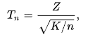
where Z is a normal random variable and K is a chi-squared random variable with n degrees of freedom. In the application, the distribution shown is obtained by dividing a normal random variable X with a chi-squared random variable with one degree of freedom.